Multi-output Sequential Data Prediction with Keras RNN model in R

   Recurrent neural networks are used to analyze sequential data. It creates the recurrent connection between the hidden units and predicts the output after learning the sequence.

   In this tutorial, we'll briefly learn how to fit and predict multi-output sequential data with the Keras RNN model in R. You can apply the same method for time-series data too. We'll use Keras R interface to implement Keras neural network API in R. The tutorial covers:

1. Preparing the data
2. Defining the model
3. Predicting and visualizing the result
4. Source code listing

We 'll start by loading the required packages of R.

library(keras)
library(caret)

Preparing the data

   First, we 'll create a multi-output dataset for this tutorial. It is randomly generated data with some rules below. There are three inputs and two outputs in this dataset. We'll plot the generated data to check it visually.

n = 850
tsize = 50

s = seq(.1, n / 10, .1)
x1 = s * sin(s / 50) - rnorm(n) * 5
x2 = s * sin(s) + rnorm(n) * 10
x3 = s * sin(s / 100) + 2 + rnorm(n) * 10
y1 = x1/2 + x2/3 + x3 + 2 + rnorm(n) 
y2 = x1 - x2 / 3 -2- x3 - rnorm(n)

df = data.frame(x1, x2, x3, y1, y2)

plot(s, df$y1, ylim = c(min(df), max(df)), type = "l", col = "blue")
lines(s, df$y2, type = "l", col = "red")
lines(s, df$x1, type = "l", col = "green")
lines(s, df$x2, type = "l", col = "yellow")
lines(s, df$x3, type = "l", col = "gray")

Next, we'll split data into the train and test parts. The last 50 elements will be the test data.

train = df[1:(n-tsize), ]
test = df[(n-tsize+1):n, ]

We'll create x input and y output data to train the model and convert them into the matrix type.

xtrain = as.matrix(data.frame(train$x1, train$x2, train$x3))
ytrain = as.matrix(data.frame(train$y1, train$y2))
xtest = as.matrix(data.frame(test$x1, test$x2, test$x3))
ytest = as.matrix(data.frame(test$y1, test$y2))

Next, we'll prepare the data by slicing the input and output values by given step value. In this example, the step value is two and we'll take the first and second rows of x and the second row of y as a label value. The next element becomes the second and the third rows of x and the third row of y, and the sequence continues until the end. The below table explains how to create the sequence of x and y data.

If the step value is 3, we'll take 3 rows of x data and the third row of y data becomes the output.

convertSeq = function(xdata, ydata, step=2) {
  y=NULL
  x =NULL
  N = dim(xdata)[1] - step
  for (i in 1:N) {

    s = i - 1 + step 

    x = abind(x, xdata[i:s,])
    y = rbind(y, ydata[s,])
  }
  x = array(x, dim = c(step, 3, N))
  return(list(x=aperm(x), y=y))
}

step=2
trains = convertSeq(xtrain, ytrain, step)
tests = convertSeq(xtest, ytest, step)

dim(trains$x)
[1] 798   3   2
dim(trains$y)
[1] 798   2

Defining the model

   We'll define the sequential model by adding the simple RNN layers, the Dense layer for output, and Adam optimizer with MSE loss function. We'll set the input dimension in the first layer and output dimension in the last layer of the model.

model = keras_model_sequential() %>%
  layer_simple_rnn(units = 32, input_shape = c(3,step), return_sequence = T) %>%
  layer_simple_rnn(units = 32) %>%
  layer_dense(units = 2)
 
model %>% compile(
  loss = "mse",
  optimizer = "adam")

model %>% summary()
______________________________________________________________________
Layer (type)                   Output Shape                Param #    
======================================================================
simple_rnn_3 (SimpleRNN)       (None, 3, 32)               1120       
______________________________________________________________________
simple_rnn_4 (SimpleRNN)       (None, 32)                  2080       
______________________________________________________________________
dense_2 (Dense)                (None, 2)                   66         
======================================================================
Total params: 3,266
Trainable params: 3,266
Non-trainable params: 0
______________________________________________________________________

We'll fit the model with train data.

model %>% fit(trains$x, trains$y, epochs = 500, batch_size = 32, verbose = 0)

And check the training accuracy.

scores = model %>% evaluate(trains$x, trains$y, verbose = 0)
print(scores)
    loss 
1.108117

Predicting and visualizing the result

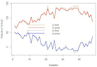
Finally, we'll predict the test data and check the accuracy of y1 and y2 with RMSE metrics.

ypred = model %>% predict(tests$x)
 

cat("y1 RMSE:", RMSE(tests$y[, 1], ypred[, 1]))
y1 RMSE: 3.379061 

cat("y2 RMSE:", RMSE(tests$y[, 2], ypred[, 2]))
y2 RMSE: 3.196091

We can check the results visually in a plot.

x_axes = seq(1:length(ypred[, 1]))

plot(x_axes, tests$y[, 1], ylim = c(min(tests$y), max(tests$y)),
     col = "burlywood", type = "l", lwd = 2,
     ylab="Outputs y1 and y2", xlab="Samples")
lines(x_axes, ypred[, 1], col = "red", type = "l", lwd = 2)
lines(x_axes, tests$y[, 2], col = "gray", type = "l", lwd = 2)
lines(x_axes, ypred[, 2], col = "blue", type = "l", lwd = 2)
legend("center", legend = c("y1-test", "y1-pred", "y2-test", "y2-pred"),
       col = c("burlywood", "red", "gray", "blue"),
       lty = 1, cex = 0.9, lwd = 2, bty = 'n')

   In this tutorial, we've briefly learned how to fit and predict multi-output sequential data with the Keras simple_rnn model in R. The full source code is listed below. 


Source code listing

library(keras)
library(caret)

n = 850
tsize = 50 

s = seq(.1, n / 10, .1)
x1 = s * sin(s / 50) - rnorm(n) * 5
x2 = s * sin(s) + rnorm(n) * 10
x3 = s * sin(s / 100) + 2 + rnorm(n) * 10
y1 = x1/2 + x2/3 + x3 + 2 + rnorm(n) 
y2 = x1 - x2 / 3 -2- x3 - rnorm(n)

df = data.frame(x1, x2, x3, y1, y2)

plot(s, df$y1, ylim = c(min(df), max(df)), type = "l", col = "blue")
lines(s, df$y2, type = "l", col = "red")
lines(s, df$x1, type = "l", col = "green")
lines(s, df$x2, type = "l", col = "yellow")
lines(s, df$x3, type = "l", col = "gray")

train = df[1:(n-tsize),]
test = df[(n-tsize+1):n,]

xtrain = as.matrix(data.frame(train$x1, train$x2, train$x3))
ytrain = as.matrix(data.frame(train$y1, train$y2))
xtest = as.matrix(data.frame(test$x1, test$x2, test$x3))
ytest = as.matrix(data.frame(test$y1, test$y2))

convertSeq = function(xdata, ydata, step=2) {
  y = NULL
  x = NULL
  N = dim(xdata)[1] - step
  for (i in 1:N) {

    s = i - 1 + step 

    x = abind(x, xdata[i:s,])
    y = rbind(y, ydata[s,])
  }
  x = array(x, dim = c(step, 3, N))
  return(list(x=aperm(x), y=y))
}

step=2
trains = convertSeq(xtrain, ytrain, step)
tests = convertSeq(xtest, ytest, step)

dim(trains$x)

dim(trains$y) 

model = keras_model_sequential() %>%
  layer_simple_rnn(units = 32, input_shape = c(3,step), return_sequence = T) %>%
  layer_simple_rnn(units = 32) %>%
  layer_dense(units = 2)
 
model %>% compile(
  loss = "mse",
  optimizer = "adam")

model %>% summary()

model %>% fit(trains$x, trains$y, epochs = 500, batch_size = 32, verbose = 0) 

scores = model %>% evaluate(trains$x, trains$y, verbose = 0)
print(scores)

ypred = model %>% predict(tests$x)
 

cat("y1 RMSE:", RMSE(tests$y[, 1], ypred[, 1])) 

cat("y2 RMSE:", RMSE(tests$y[, 2], ypred[, 2]))

x_axes = seq(1:length(ypred[, 1]))

plot(x_axes, tests$y[, 1], ylim = c(min(tests$y), max(tests$y)),
     col = "burlywood", type = "l", lwd = 2,
     ylab="Outputs y1 and y2", xlab="Samples")
lines(x_axes, ypred[, 1], col = "red", type = "l", lwd = 2)
lines(x_axes, tests$y[, 2], col = "gray", type = "l", lwd = 2)
lines(x_axes, ypred[, 2], col = "blue", type = "l", lwd = 2)
legend("center", legend = c("y1-test", "y1-pred", "y2-test", "y2-pred"),
       col = c("burlywood", "red", "gray", "blue"),
       lty = 1, cex = 0.9, lwd = 2, bty = 'n')