Smoothing Example with Savitzky-Golay Filter in Python

     The Savitzky-Golay filter is a widely-used technique in signal processing aimed at reducing noise and enhancing the smoothness of signal trends. This filter achieves this by computing a polynomial fit for each window, with parameters such as polynomial degree and window size influencing the smoothing process.

    The SciPy library offers the savgol_filter() function, which facilitates the implemention of the Savitzky-Golay filter. In this tutorial, we'll provide an overview of utilizing the savgol_filter() function to effectively smooth signal data in Python.. 

    The tutorial covers:

1. Preparing signal data
2. Smoothing with the Savitzky-Golay filter
3. Source code listing
   

    We'll start by loading the required libraries.

import numpy as np
from scipy import signal
import matplotlib.pyplot as plt 

Preparing signal data

 

    To begin, we'll generate signal data for this tutorial and visualize it on a graph.

 

x = np.arange(-2, 2, 0.02)
y = np.array(x**2 + 2*np.sin(x*np.pi)) 
y = y + np.array(np.random.random(len(x)) * 2.3)

plt.figure(figsize=(12, 9))

plt.plot(x, y, label="y_signal")
plt.legend()
plt.grid(True)
plt.show()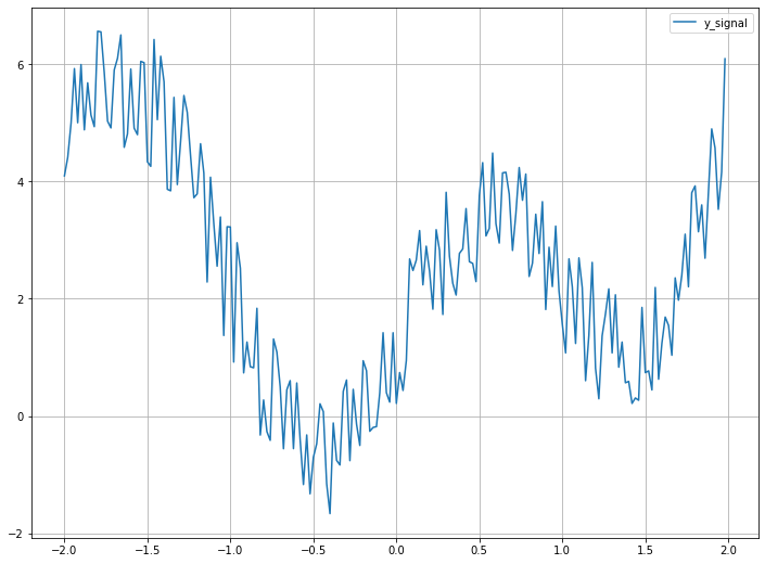 

 

    Our task is to smooth above signal by using  savgol_filter() function.

 

 

Smoothing with Savitzky-Golay filter

 

    The Savitzky-Golay filter is a digital signal processing technique used for smoothing and noise reduction in signal or time-series  data. It's particularly effective for preserving the features of the signal while removing unwanted noise. 

    To smooth the signal data, the Savitzky-Golay filter calculates a polynomial fit for each window based on the specified polynomial degree and window size. The SciPy function savgol_filter() in the signal module is commonly used for applying the Savitzky-Golay filter to one-dimensional arrays of data. This function requires a one-dimensional array of data, the window length (typically an odd integer), the polynomial order, and optionally, other parameters such as the order of the derivative to compute. These parameters can be set as shown below:

 

y_smooth = signal.savgol_filter(y, window_length=11, polyorder=3, mode="nearest")

    The mode parameter in the savgol_filter() function is optional and determines the type of extension to use for the padded signal to which the filter is applied. The mode can be defined as one of the following types: 'mirror', 'nearest', 'constant', and 'wrap'. You can choose the appropriate mode based on the characteristics of your data and the desired behavior at the signal boundaries. More details about each mode and other optional parameters of the function can be found in the SciPy reference page.

    After applying the Savitzky-Golay filter to the data, we visualize the smoothed data in a graph to observe the effect of the smoothing operation.

plt.figure(figsize=(12, 9))
plt.plot(x, y, label="y_signal")
plt.plot(x, y_smooth, linewidth=3, label="y_smoothed")
plt.legend()
plt.grid(True)
plt.show() 

    Now we adjust the window size and polynomial order parameters to effectively smooth the trend of a signal. In this example, we'll experiment with multiple window sizes to observe their smoothing effects on a given dataset.

ig, ax = plt.subplots(4, figsize=(8, 14))
i = 0 
# define window sizes 5, 11, 21, 31
for w_size in [5, 11, 21, 31]:    
    y_fit = signal.savgol_filter(y, w_size, 3, mode="nearest")
    ax[i].plot(x, y, label="y_signal", color="green")
    ax[i].plot(x, y_fit, label="y_smoothed", color="red")
    ax[i].set_title("Window size: " + str(w_size))
    ax[i].legend()
    ax[i].grid(True)
    i+=1

plt.tight_layout()        
plt.show() 

 

 

    In the graph above, we observe how adjusting the window size impacts the smoothness of the signal trend. This flexibility allows us to determine the optimal window size for our specific dataset.

 

    In this tutorial, we've explored the process of smoothing signal data using the savgol_filter() function in Python. The Savitzky-Golay filter provides a simple yet powerful method for smoothing and denoising signal data. Below is the complete source code for reference.

 

Source code listing

import numpy as np
from scipy import signal
import matplotlib.pyplot as plt

x = np.arange(-2, 2, 0.02)
y = np.array(x**2+2*np.sin(x*np.pi)) 
y = y + np.array(np.random.random(len(x))*2.3)

plt.figure(figsize=(12, 9))

plt.plot(x, y, label="y_signal")
plt.legend()
plt.grid(True)
plt.show()

y_smooth = signal.savgol_filter(y, window_length=11, polyorder=3, mode="nearest")
    
plt.figure(figsize=(12, 9))
plt.plot(x, y, label="y_signal")
plt.plot(x, y_smooth, linewidth=3, label="y_smoothed")
plt.legend()
plt.grid(True)
plt.show()

ig, ax = plt.subplots(4, figsize=(8, 14))
i = 0

 
# define window sizes 5, 11, 21, 31
for w_size in [5, 11, 21, 31]:    
    y_fit = signal.savgol_filter(y, w_size, 3, mode="nearest")
    ax[i].plot(x, y, label="y_signal", color="green")
    ax[i].plot(x, y_fit, label="y_smoothed", color="red")
    ax[i].set_title("Window size: " + str(w_size))
    ax[i].legend()
    ax[i].grid(True)
    i+=1

plt.tight_layout()        
plt.show() 

 

 

References:

1. SciPy Savitzky-Golay filter