Applying the Stochastic
Gradient Descent (SGD) method to the linear classifier or regressor provides the efficient
estimator for classification and regression problems.
Scikit-learn API provides the SGDRegressor class to implement SGD method for regression problems. The SGD regressor applies regularized linear model with SGD learning to build an estimator. A regularizer is a penalty (L1, L2, or Elastic Net) added to the loss function to shrink the model parameters. The SGD regressor works well with large-scale datasets.
In previous post, we learned how to classify data with SGD classifier in Python and you can find it here.
In this tutorial, we'll briefly learn how to fit and predict regression data by using
Scikit-learn's SGDRegressor class in Python. The tutorial
covers:
- Preparing the data
- Training the model
- Predicting and accuracy check
- Boston dataset prediction
- Source code listing
from sklearn.linear_model import SGDRegressor
from sklearn.datasets import load_boston
from sklearn.datasets import make_regression
from sklearn.metrics import mean_squared_error
from sklearn.model_selection import train_test_split
from sklearn.model_selection import cross_val_score
from sklearn.preprocessing import scale
import matplotlib.pyplot as plt
Preparing the data
First,
we'll generate random regression data with make_regression()
function. The dataset contains 30 features and 1000 samples.
To improve the model accuracy we'll scale both x and y data then, split them into train and test parts. Here, we'll extract 15 percent of the samples as test data.
x, y = make_regression(n_samples=1000, n_features=30)
To improve the model accuracy we'll scale both x and y data then, split them into train and test parts. Here, we'll extract 15 percent of the samples as test data.
x = scale(x)
y = scale(y)
xtrain, xtest, ytrain, ytest=train_test_split(x, y, test_size=0.15)
Training the model
Next, we'll define the regressor model by using the SGDRegressor
class. Here, we can use default parameters of the SGDRegressor class.
sgdr = SGDRegressor()
print(sgdr)
Then, we'll fit the model on train data and check the model accuracy score.
sgdr.fit(xtrain, ytrain)

score = sgdr.score(xtrain, ytrain)
print("R-squared:", score)

R-squared: 0.9999999253180197
We can also apply a cross-validation method to the model and check the training accuracy.
cv_score = cross_val_score(sgdr, x, y, cv = 10)
print("CV mean score: ", cv_score.mean())

CV mean score:  0.9999999624822019
Predicting and accuracy check
Now, we can predict the test data by using the trained model. We can
check the accuracy of predicted data by using MSE and RMSE metrics.
ypred = sgdr.predict(xtest)

mse = mean_squared_error(ytest, ypred)
print("MSE: ", mse)
print("RMSE: ", mse**(1/2.0))
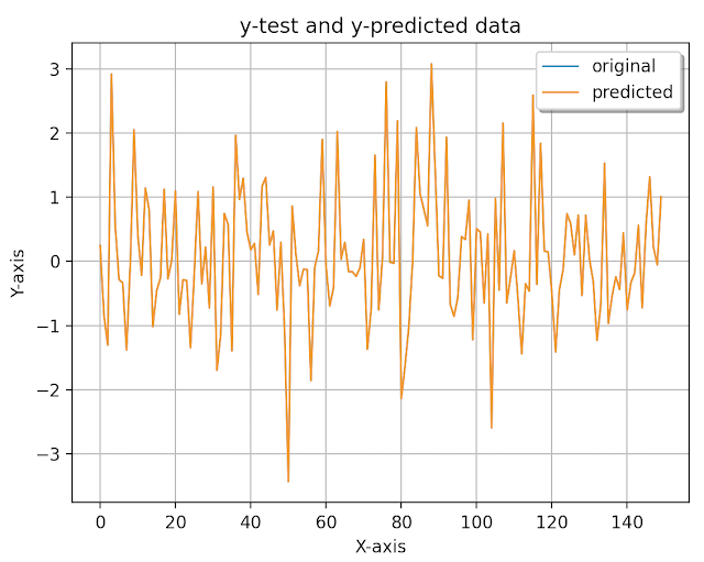
MSE: 1.1979434697284535e-07
RMSE: 5.989717348642267e-08
Finally, we'll visualize the original and predicted data in a plot.
x_ax = range(len(ytest))
plt.plot(x_ax, ytest, linewidth=1, label="original")
plt.plot(x_ax, ypred, linewidth=1.1, label="predicted")
plt.title("y-test and y-predicted data")
plt.xlabel('X-axis')
plt.ylabel('Y-axis')
plt.legend(loc='best',fancybox=True, shadow=True)
plt.grid(True)
plt.show()
Boston housing dataset prediction
We'll
apply the same method we've learned above to the Boston housing price
regression dataset. We'll load it by using load_boston() function, scale
and split into train and test parts. Then, we'll define model by changing some of the parameter values, check training accuracy, and predict test data.
print("Boston housing dataset prediction.")
boston = load_boston()
x, y = boston.data, boston.target

x = scale(x)
y = scale(y)
xtrain, xtest, ytrain, ytest = train_test_split(x, y, test_size=.15)

sgdr = SGDRegressor(alpha=0.0001, epsilon=0.01, eta0=0.1,penalty='elasticnet')
sgdr.fit(xtrain, ytrain)

score = sgdr.score(xtrain, ytrain)
print("R-squared:", score)

# cv_score = cross_val_score(lsvr, x, y, cv=5)
# print("CV mean score: ", cv_score.mean())

ypred = sgdr.predict(xtest)

mse = mean_squared_error(ytest, ypred)
print("MSE: ", mse)
print("RMSE: ", mse**(1/2.0))

x_ax = range(len(ytest))
plt.plot(x_ax, ytest, label="original")
plt.plot(x_ax, ypred, label="predicted")
plt.title("Boston test and predicted data")
plt.xlabel('X-axis')
plt.ylabel('Y-axis')
plt.legend(loc='best',fancybox=True, shadow=True)
plt.grid(True)
plt.show()
Boston housing dataset prediction.
R-squared: 0.7239074887406243
MSE:  0.2200176437469965
RMSE:  0.11000882187349825
In this tutorial, we've briefly learned how to fit and predict regression data by using
Scikit-learn API's SGDRegressor class in Python. The full
source code is listed below.
Source code listing
from sklearn.linear_model import SGDRegressor
from sklearn.datasets import load_boston
from sklearn.datasets import make_regression
from sklearn.metrics import mean_squared_error
from sklearn.model_selection import train_test_split
from sklearn.model_selection import cross_val_score
from sklearn.preprocessing import scale
import matplotlib.pyplot as plt

x, y = make_regression(n_samples=1000, n_features=30)
print(x[0:2])
print(y[0:2])

x = scale(x)
y = scale(y)
xtrain, xtest, ytrain, ytest = train_test_split(x, y, test_size=.15)

sgdr = SGDRegressor()
print(sgdr)

sgdr.fit(xtrain, ytrain)

score = sgdr.score(xtrain, ytrain)
print("R-squared:", score)

cv_score = cross_val_score(sgdr, x, y, cv=10)
print("CV mean score: ", cv_score.mean())

ypred = sgdr.predict(xtest)

mse = mean_squared_error(ytest, ypred)
print("MSE: ", mse)
print("RMSE: ", mse**(1/2.0))

x_ax = range(len(ytest))
plt.plot(x_ax, ytest, linewidth=1, label="original")
plt.plot(x_ax, ypred, linewidth=1.1, label="predicted")
plt.title("y-test and y-predicted data")
plt.xlabel('X-axis')
plt.ylabel('Y-axis')
plt.legend(loc='best',fancybox=True, shadow=True)
plt.grid(True)
plt.show()


print("Boston housing dataset prediction.")
boston = load_boston()
x, y = boston.data, boston.target

x = scale(x)
y = scale(y)
xtrain, xtest, ytrain, ytest = train_test_split(x, y, test_size=.15)

sgdr = SGDRegressor(alpha=0.0001, epsilon=0.01, eta0=0.1,penalty='elasticnet')
sgdr.fit(xtrain, ytrain)

score = sgdr.score(xtrain, ytrain)
print("R-squared:", score)


ypred = sgdr.predict(xtest)

mse = mean_squared_error(ytest, ypred)
print("MSE: ", mse)
print("RMSE: ", mse**(1/2.0))

x_ax = range(len(ytest))
plt.plot(x_ax, ytest, label="original")
plt.plot(x_ax, ypred, label="predicted")
plt.title("Boston test and predicted data")
plt.xlabel('X-axis')
plt.ylabel('Y-axis')
plt.legend(loc='best',fancybox=True, shadow=True)
plt.grid(True)
plt.show()
References:


are you missing an asterisk? `print("RMSE: ", mse*(1/2.0))`
ReplyDeleteYes, and corrected it.
DeleteWhat is nsvr? It is referenced calling the predict method, I'm assuming it's supposed to be sgdr.
ReplyDeleteyes, it is sgdr
DeleteHello, Thanks for this amazing tutorial! I've a question: How we can deal with one-hot encoded features? should we scale them too?
ReplyDeleteI wanted to get the coefficients as well as bias of the model. I did the following
ReplyDeletemodel = SGDRegressor(random_state=0)
model.fit(x_train, y_train.ravel())
print('coef are ',sgd_fit.coef_)
print('bias is',sgd_fit.intercept_)
print("coef are", model.coef_)
Deletemodel = SGDRegressor(random_state=0)
ReplyDeletemodel.fit(x_train, y_train.ravel())
# print(sgd_fit)
#print(sgd_fit.predict(np.zeros((1,8))))
print('coef are ',sgd_fit.coef_)
print('bias is',sgd_fit.intercept_)